The following plots compare the performance of moocore
against emoa, targeted
and caRamel.
Other R packages are not included in the comparison because they are
based on these packages for the functionality benchmarked, so they are
at least as slow as them. For example, GPareto
and rmoo use
emoa
to compute the hypervolume. bbotk
already uses moocore.
Not all packages provide the same functionality.
Show benchmarking setup code
library(matrixStats)
library(data.table)
#>
#> Attaching package: 'data.table'
#> The following object is masked from 'package:base':
#>
#>     %notin%
library(ggplot2)
library(moocore)

geomspace <- function(start, stop, num) {
  x <- round(10^(seq(log10(start), log10(stop), length.out = num)), 0)
  x[1] <- start
  x[length(x)] <- stop
  x
}

read_ndset <- function(filename, filter=FALSE) {
  cat("Get file '", filename, "'\n")
  destfile <- system.file(file.path("extdata", filename), package="moocore")
  if (destfile == "") {
    destfile <- file.path("../../../testsuite/data", filename)
    if (!file.exists(destfile)) {
      fileext <- if (endsWith(destfile, ".xz")) ".xz" else ""
      destfile <- withr::local_tempfile(fileext = fileext)
      base_url <- "https://github.com/multi-objective/testsuite/raw/refs/heads/main/data/"
      utils::download.file(paste0(base_url, filename), destfile, quiet = FALSE)
    }
  }
  x <- read_datasets(destfile)
  x <- x[, -ncol(x)] # Union of datasets
  if (filter)
    x <- filter_dominated(x)
  x
}

# This is adapted from atime:::plot.atime
benchmark_plot <- function (x, title = "", only_seconds=TRUE, ...) {
  expr.name <- N <- kilobytes <- NULL
  meas <- x[["measurements"]]
  by.dt <- meas[, x$by.vec, with = FALSE]
  tall.list <- list()
  for (unit.i in seq_along(x$unit.col.vec)) {
    col.name <- x$unit.col.vec[[unit.i]]
    unit <- names(x$unit.col.vec)[[unit.i]]
    if (is.null(unit) || unit == "")
      unit <- col.name
    tall.list[[unit.i]] <- meas[, data.table(N, by.dt,
      unit, median = get(col.name))]
  }
  tall <- rbindlist(tall.list)
  if (only_seconds) {
    tall <- tall[unit=="seconds", ]
    ylab <- "CPU time (seconds)"
  } else {
    ylab <- "median line, min/max band"
  }

  gg <- ggplot() + theme_bw(base_size=12) +
    geom_ribbon(aes(N, ymin = min, ymax = max, fill = expr.name),
      data = data.table(meas, unit = "seconds"), alpha = 0.25, show.legend=FALSE) +
    geom_line(aes(N, median, color = expr.name), data = tall) +
    geom_point(aes(N, median, color = expr.name), data = tall) +
    scale_x_log10(breaks = unique(tall$N), labels = unique(tall$N)) +
    scale_y_log10(ylab, labels = scales::label_log(), guide="axis_logticks") +
    labs(subtitle = title) +
    theme(axis.text.x = element_text(angle = 45, vjust = 1, hjust = 1))
  if (only_seconds) {
    gg <- gg + theme(legend.title = element_blank(),
      legend.background = element_rect(fill=alpha("white", alpha=0.5)),
      legend.key = element_rect(fill = NA, color = NA),
      legend.position = "inside",
      legend.position.inside = c(0.99, 0.01),
      legend.justification = c("right", "bottom"),
      legend.margin = margin_auto(0))
  } else {
    gg <- gg + theme(legend.title = element_blank(),
      legend.background = element_rect(fill=alpha("white", alpha=0.5)),
      legend.position = c(0.8, 0.625)) + facet_grid(unit ~ ., scales = "free")
  }
  gg
}

get_package_version <- function(package)
  paste0(package, " (", as.character(packageVersion(package)), ")")

benchmark <- function(name, x, N, setup, expr.list, prefix, title, check)
{
  rds_file <- paste0("bench/bench-", prefix, "-", name, ".rds")
  if (run_benchmarks || !file.exists(rds_file)) {
    lapply(names(expr.list), library, character.only = TRUE)
    names(expr.list) <- sapply(names(expr.list), get_package_version, USE.NAMES=FALSE)
    if (!requireNamespace("atime", quietly = TRUE)
      || packageVersion("atime") < "2026.7.1") {
      stop("Please install atime >= 2026.7.1")
    }
    res <- substitute(atime::atime(
      N = N,
      expr.list = expr.list,
      setup = SETUP,
      result=FALSE,
      times=5,
      check=check,
      seconds.limit=10), list(SETUP=setup))
    res <- eval(res)
    saveRDS(res, file = rds_file)
  } else {
    res <- readRDS(rds_file)
  }
  gg <- benchmark_plot(res, title = paste0(title, " for ", name))
  gg
}

get_ndset <- function(x, filter)
{
  if (is.null(x$generate)) return(read_ndset(x$file, filter=filter))
  do.call(moocore::generate_ndset, x$generate)
}

benchmark_all <- function(files, prefix, title, setup, expr.list, filter, check=TRUE)
{
  for (name in names(files)) {
    p <- benchmark(name = name, x = get_ndset(files[[name]], filter=filter),
      N = files[[name]]$N, prefix = prefix, title = title,
      setup = setup,  expr.list = expr.list, check=check)
    print(p)
  }
}
Identifying (non)dominated points
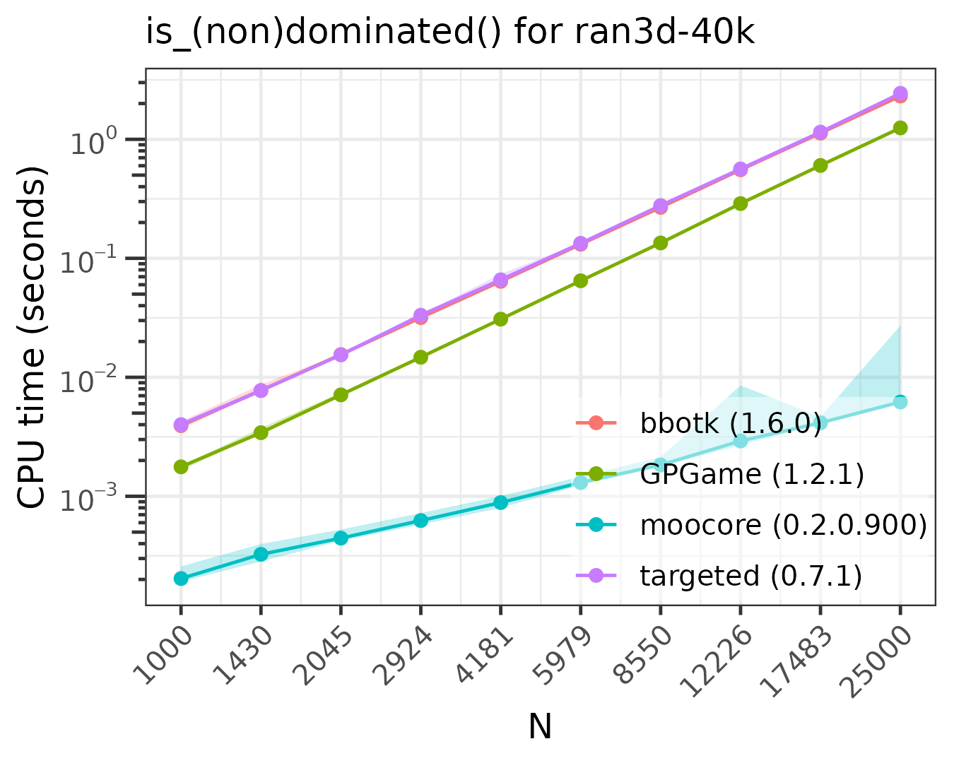
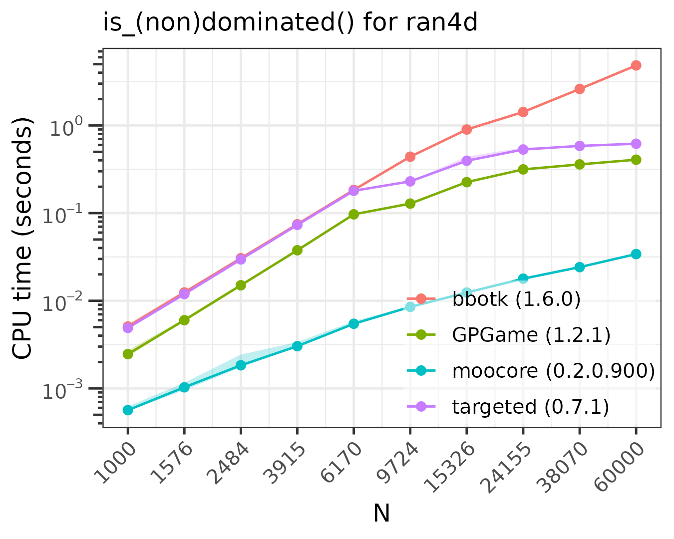
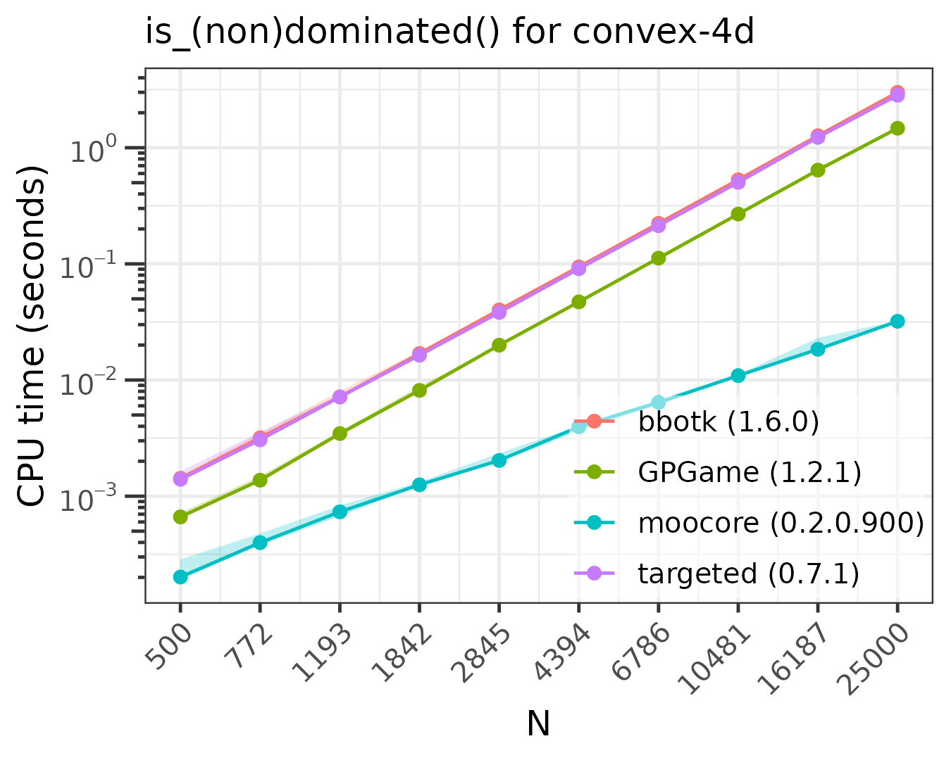
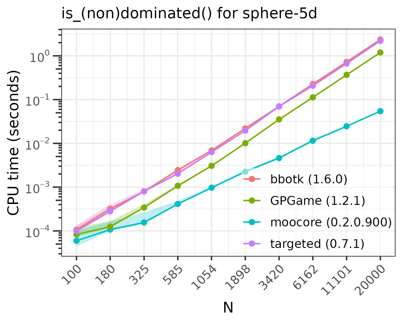
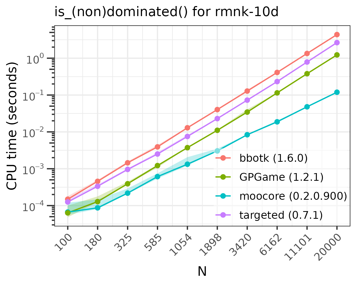
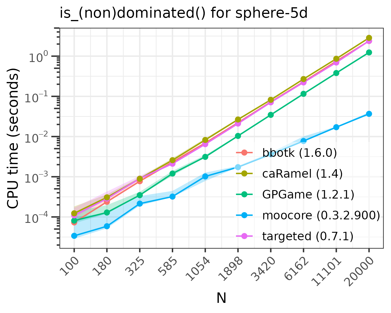
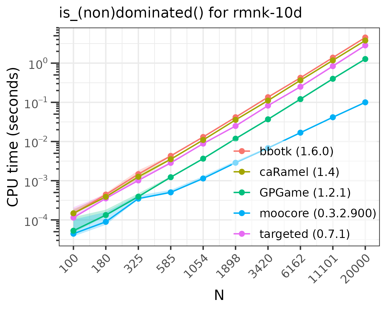
The following plots compare the speed of finding (non)dominated
solutions, equivalent to moocore::is_nondominated(), in 2D,
3D, 4D, 5D and 10D. The plots show that moocore
is always 10 times faster than GPGame,
caRamel
and targeted
for any number of objectives. In addition, GPGame
calculates wrong values with repeated coordinates (vpicheny/GPGame#2).
The rand4d testcase is somewhat different from the others,
as it is mostly composed of dominated points (only 10590 points are
nondominated), while the other testcases are mostly nondominated
sets.
setup <- quote({
  stopifnot(nrow(x) >= N)
  z <- as.matrix(x[1L:N, ])
  nz <- -z
  tz <- t(z)
  gc() # clean state before timing
})

expr.list <- list(
  moocore = quote(which(moocore::is_nondominated(z))),
  GPGame = quote(GPGame::nonDom(z)),
  targeted = quote(targeted::nondom(z)),
  caRamel = quote(caRamel::pareto(nz))
)

files <- list(
  "test2D-200k"=list(file="test2D-200k.inp.xz", N=geomspace(1000, 50000, 10)),
  "ran3d-40k"=list(file="ran.40000pts.3d.1.xz", N=geomspace(1000, 25000, 10)),
  "convex-3d"=list(generate=list(25000, 3, "convex-sphere", 42), N=geomspace(1000, 25000, 10)),
  "sphere-3d"=list(generate=list(25000, 3, "sphere", 42), N=geomspace(1000, 25000, 10)),
  "ran4d"=list(file="ran.9000pts.4d.10.xz", N=geomspace(1000, 60000, 10)),
  "convex-4d"=list(generate=list(25000, 4, "convex-sphere", 42), N=geomspace(500, 25000, 10)),
  "sphere-5d"=list(generate=list(20000, 5, "sphere", 42), N=geomspace(100, 20000, 10)),
  "rmnk-10d"=list(file="rmnk_0.0_10_16_1_0_ref.txt.xz", N=geomspace(100, 20000, 10))
)

benchmark_all(files, prefix="ndom", title = "is_(non)dominated()",
  setup = setup, expr.list = expr.list, filter=FALSE, check=FALSE)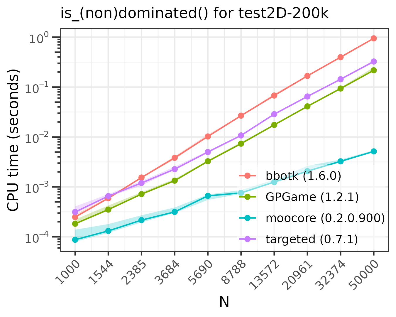
Exact computation of hypervolume
The following plots compare the speed of computing the hypervolume indicator in 3D, 4D, 5D and 6D.
setup <- quote({
  ref <- colMaxs(x, useNames = FALSE) + 1L
  stopifnot(nrow(x) >= N)
  z <- x[1L:N, ]
  tz <- t(z)
  gc() # clean state before timing
})

expr.list <- list(
  moocore = quote(moocore::hypervolume(z, ref = ref)),
  emoa = quote(emoa::dominated_hypervolume(tz, ref = ref)))

files <- list(
  "spherical-3d"=list(
    file = "spherical-3d-2000pts-10.dat.xz",
    N = geomspace(100, 20000, 10)),
  "DTLZLinearShape.4d"=list(
    file = "DTLZLinearShape.4d.front.1000pts.10",
    N = geomspace(100, 2000, 10)),
  "DTLZLinearShape.5d"=list(
    file = "DTLZLinearShape.5d.front.500pts.10",
    N = geomspace(100, 1000, 10)),
  "DTLZLinearShape.6d"=list(
    file = "DTLZLinearShape.6d.front.700pts.10.xz",
    N = geomspace(100, 1000, 10))
)

benchmark_all(files, prefix="hv", title = "HV Computation",
  setup = setup, expr.list = expr.list, filter=TRUE)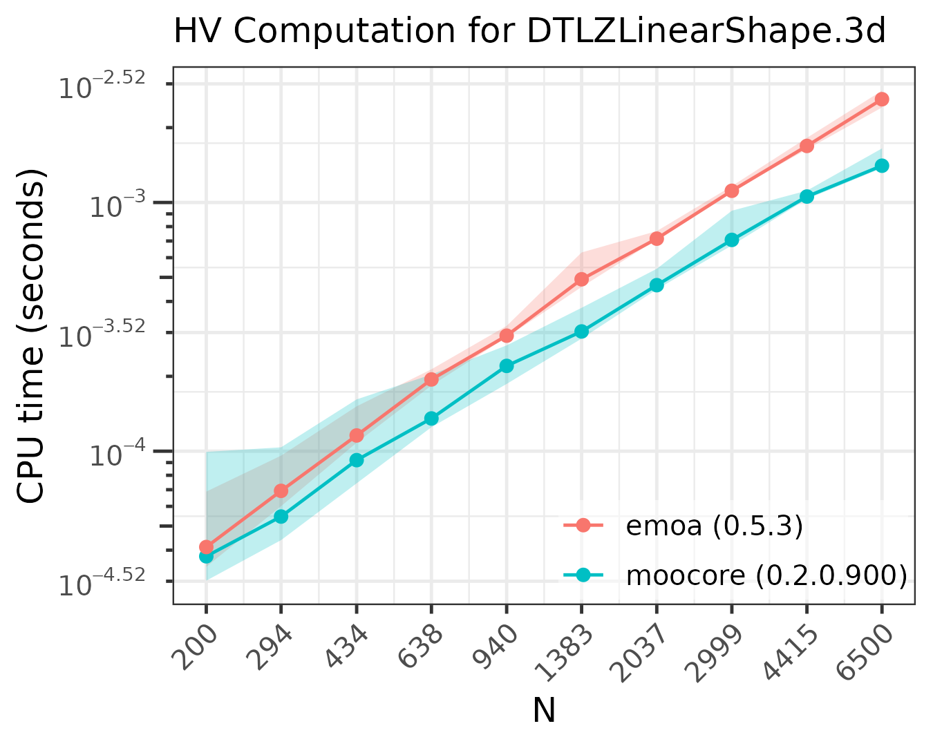
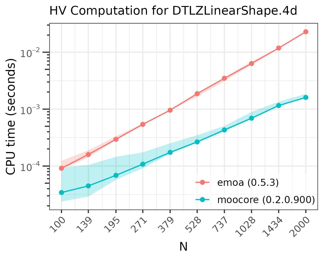
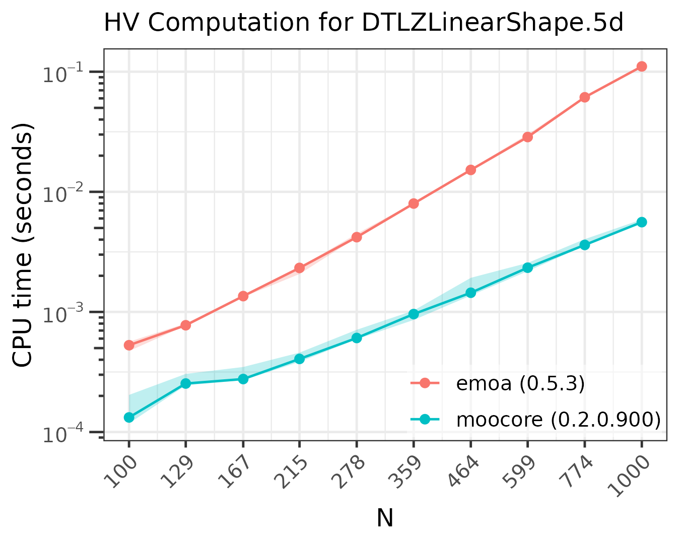
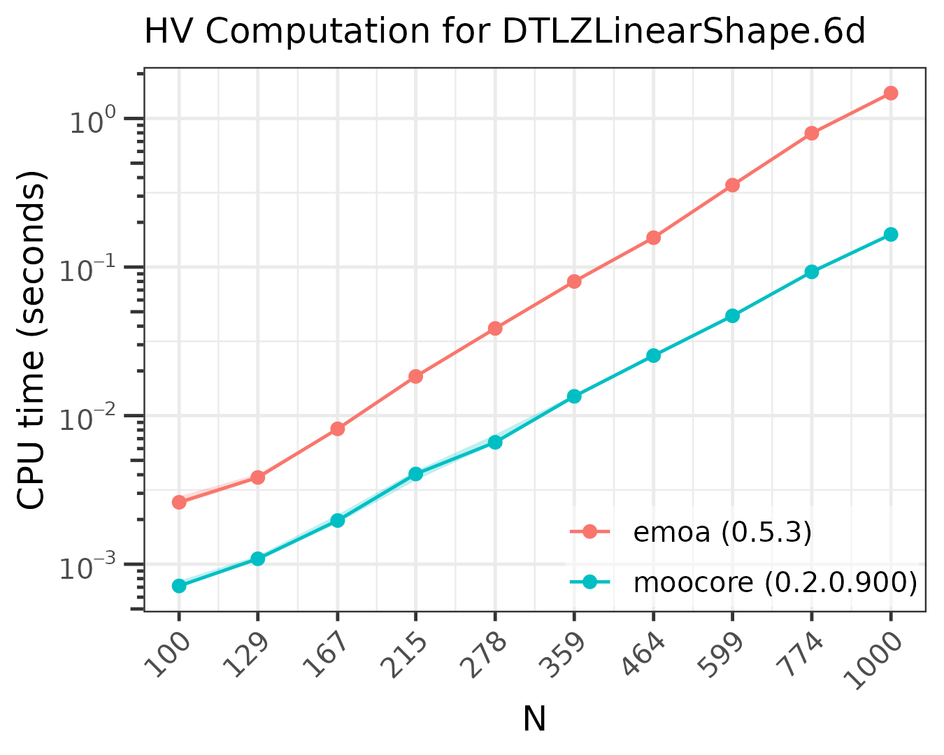
As the plots show, moocore
is always faster than emoa
and, hence, faster than GPareto
and rmoo.
Hypervolume contribution
The only R package, other than moocore,
able to compute hypervolume contributions
moocore::hv_contributions() is emoa.
However, emoa is
buggy and calculates wrong values (olafmersmann/emoa#1).