Approximating the hypervolume

library(moocore)
library(dplyr, warn.conflicts=FALSE)

The following examples compare various ways of approximating the hypervolume of a nondominated set.

Comparing HypE and Rphi-FWE+

This example shows how to approximate the hypervolume metric of the CPFs.txt dataset using both whv_hype() (HypE), and hv_approx() for several values of the number of samples between $10^1$ and $10^5$. We repeat each calculation 5 times to account for stochasticity.

First calculate the exact hypervolume.

ref <- 2.1
data(CPFs)
x <- filter_dominated(CPFs[,1:2])
x <- normalise(x, to_range=c(1, 2))
true_hv <- hypervolume(x, reference = ref)
true_hv
#> [1] 1.057045

Next, we approximate the hypervolume using $\{10^1, 10^2, \ldots, 10^5\}$ random samples to show the higher samples reduce the approximation error. Since the approximation is stochastic, we perform 5 repetitions of each computation.

nreps <- 5
nsamples_exp <- 5
set.seed(42)
results <- list("HypE" = list(), "DZ2019-HW" = list(), "DZ2019-MC" = list(), "Rphi-FWE+" = list())
df <- data.frame(Method=character(), rep=integer(), samples=numeric(), value=numeric())

for (i in seq_len(nsamples_exp)) {
  df <- rbind(df,
    # We use rep=c(1,1) to silence a ggplot2 warning with mean_cl_boot.
    data.frame(Method="DZ2019-HW", rep=c(1,1), samples=10^i,
      value = hv_approx(x, reference = ref, nsamples = 10^i, method="DZ2019-HW")),
    data.frame(Method="Rphi-FWE+", rep=c(1,1), samples=10^i,
      value = hv_approx(x, reference = ref, nsamples = 10^i, method="Rphi-FWE+")),
    data.frame(Method="HypE", rep=seq_len(nreps), samples=10^i,
      value = sapply(seq_len(nreps), function(r)
        whv_hype(x, reference = ref, ideal = 0, nsamples = 10^i, seed = 42 + r))),
    data.frame(Method="DZ2019-MC", rep=seq_len(nreps), samples=10^i,
      value = sapply(seq_len(nreps), function(r)
        hv_approx(x, reference = ref, nsamples = 10^i, seed = 42 + r, method="DZ2019-MC")))
    )
}
df[["error"]] <- abs(df[["value"]] - true_hv) / true_hv
res <- df %>% filter(samples == max(samples)) %>% group_by(Method) %>%
  summarise(Mean = mean(value), Min = min(value), Max = max(value))
width <- nchar("Mean of DZ2019-MC")
text <- c(sprintf("%*s : %.12f", width, "True HV", true_hv),
  sapply(res$Method, function(method)
  sprintf("%*s : %.12f  [min, max] = [%.12f, %.12f]", width,
    paste0("Mean of ", method),
    res[res$Method == method, "Mean"],
    res[res$Method == method, "Min"],
    res[res$Method == method, "Max"])))
cat(sep="\n", text)
#>           True HV : 1.057044746430
#> Mean of DZ2019-HW : 1.057044746450  [min, max] = [1.057044746450, 1.057044746450]
#> Mean of DZ2019-MC : 1.057233221522  [min, max] = [1.056868277766, 1.057665468167]
#>      Mean of HypE : 1.058779259998  [min, max] = [1.055621699998, 1.063736099998]
#> Mean of Rphi-FWE+ : 1.057042456377  [min, max] = [1.057042456377, 1.057042456377]

Next, we plot the results.

library(ggplot2)
library(scales)
ggplot(df, aes(samples, error, color=Method)) +
  stat_summary(fun = mean, geom = "line") +
  stat_summary(fun.data = mean_cl_boot, geom = "ribbon", color = NA, alpha=0.2,
    mapping=aes(fill=Method)) +
  scale_x_log10(labels = label_log()) +
  scale_y_log10(labels = label_log()) +
  labs(x = "Samples", y = "Relative Error") +
  theme_bw()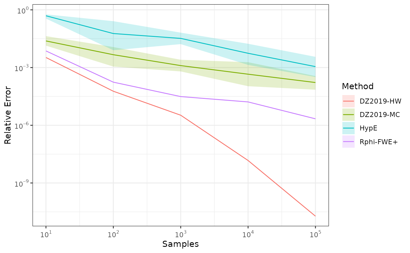

Comparing Monte-Carlo and quasi-Monte-Carlo approximations

The quasi-Monte-Carlo approximations with method=Rphi-FWE+ (López-Ibáñez 2026) and method=DZ2019-HW (Deng and Zhang 2019) are deterministic, but not monotonic on the number of samples. Nevertheless, they are often better than the Monte-Carlo approximation generated with method=DZ2019-MC (Deng and Zhang 2019), specially with large number of objectives. A more detailed comparison is provided by López-Ibáñez (2026).

library(moocore)
library(ggplot2)
library(scales)
datasets <- c("DTLZLinearShape.8d.front.60pts.10", "ran.10pts.9d.10")
ref <- 10
samples <- 2 ** (12:18)
maxiter <- max(samples)
nreps <- 5
df <- NULL
for (dataset in datasets) {
  x <- read_datasets(system.file(file.path("extdata", dataset),
    package="moocore", mustWork=TRUE))
  x <- x[, -ncol(x)] # Union of datasets.
  x <- filter_dominated(x)[1:10, ]
  exact <- hypervolume(x, reference=ref)
  res <- list(
    data.frame(Method="DZ2019-HW", samples = samples, seed = NA,
      hv = sapply(samples, function(i)
        hv_approx(x, reference=ref, nsamples=i, method="DZ2019-HW"))),
    data.frame(Method="Rphi-FWE+", samples = samples, seed = NA,
      hv = sapply(samples, function(i)
        hv_approx(x, reference=ref, nsamples=i, method="Rphi-FWE+"))))
  # Duplicate the observations to avoid a warning with mean_cl_boot
  res <- c(res, res)
  for (k in seq_len(nreps)) {
    seed <- 42 + k
    res <- c(res, list(
      data.frame(Method="DZ2019-MC", samples = samples, seed = seed,
        hv = sapply(samples, function(i)
          hv_approx(x, reference=ref, nsamples=i, method="DZ2019-MC", seed=seed)))))
  }
  res <- do.call("rbind", res)
  res[["hverror"]] <- abs(1.0 - (res$hv / exact))
  res[["dataset"]] <- dataset
  df <- rbind(df, res)
}
ggplot(df, aes(x = samples, y = hverror, color = Method)) +
  stat_summary(fun = mean, geom = "line") +
  stat_summary(fun = mean, geom = "point") +
  stat_summary(fun.data = mean_cl_boot, geom = "ribbon", color = NA, alpha=0.2,
    mapping=aes(fill=Method)) +
  scale_y_log10(labels = label_log(), breaks = 10^(-5:5)) +
  scale_x_continuous(trans = "log2", labels = label_log(base=2)) +
  labs(x = "Samples", y = "Relative error") +
  facet_wrap(~dataset, scales="free_y",nrow=2) +
  theme_bw()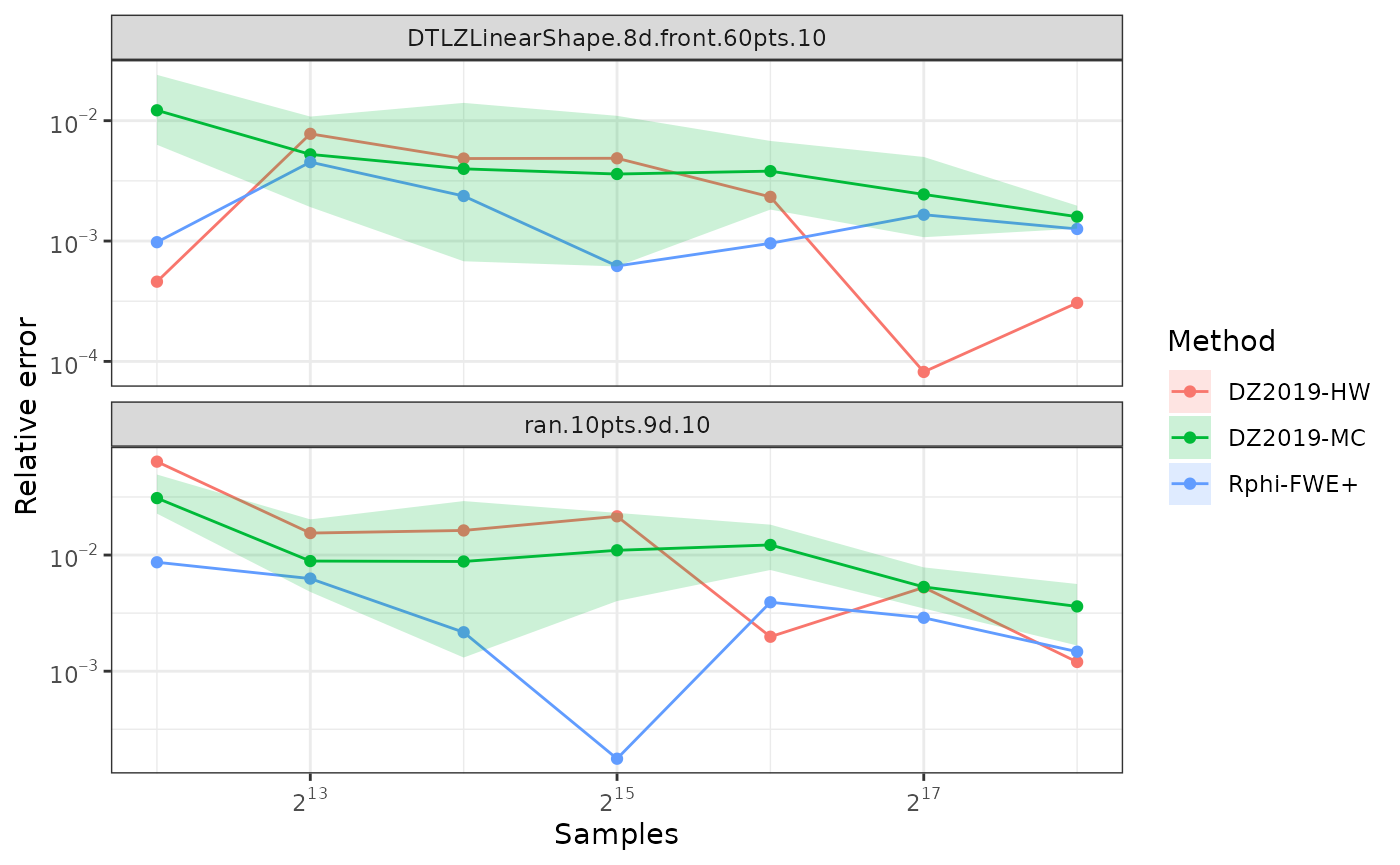

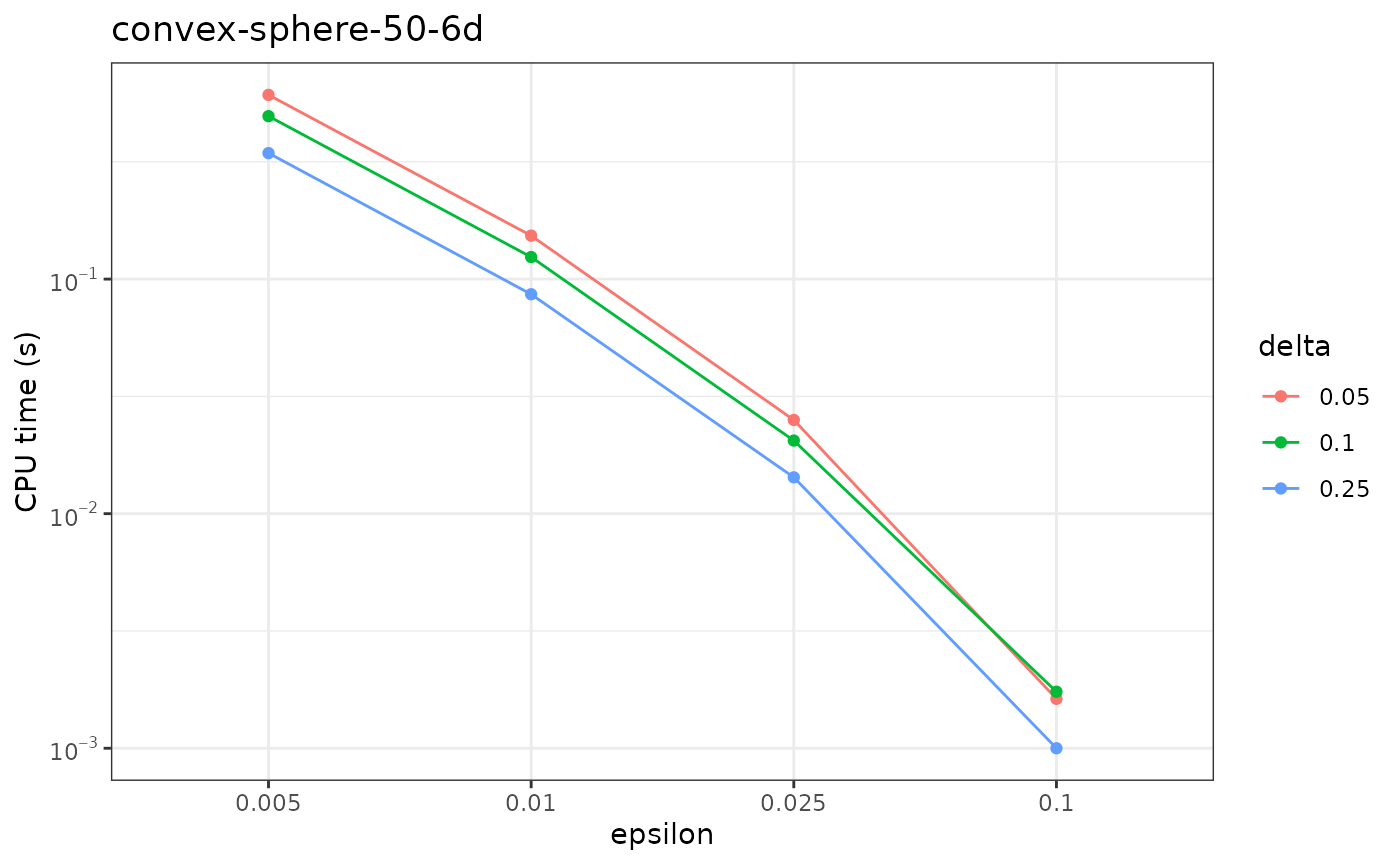
FPRAS: Fully Polynomial-Time Randomized Approximation Scheme

hv_approx_fpras() allows obtaining an approximation with relative error smaller than $\epsilon$ (epsilon) with a given probability $1-\delta$ (delta). As the plot below shows, the approximation error is often better than the requested value, but the computation time increases very quickly for smaller epsilon.

library(ggplot2)
library(scales)
shape <- "convex-sphere"
ref <- 1.1
npoints <- 50
dim <- 6
nreps <- 10
set.seed(42)
res <- NULL
for (r in seq_len(nreps)) {
  z <- generate_ndset(npoints, dim, method = shape, seed = 42 + r)
  exact <- hypervolume(z, reference = ref)
  for (epsilon in c(0.1, 0.025, 0.01, 0.005)) {
    for (delta in c(0.25, 0.1, 0.05)) {
      t_start <- proc.time()[["elapsed"]]
      hv <- hv_approx_fpras(z, reference = ref, epsilon = epsilon, delta = delta)
      t_end <- proc.time()[["elapsed"]] - t_start
      res <- rbind(res, data.frame(
        r = r,
        epsilon = epsilon,
        delta = delta,
        hverror = abs(1 - hv / exact),
        time = t_end
      ))
    }
  }
}
res[["delta"]] <- as.factor(res[["delta"]])
res[["epsilon"]] <- as.factor(res[["epsilon"]])

ggplot(res, aes(x = epsilon, y = hverror, fill = delta)) +
  geom_boxplot() +
  scale_y_log10(labels = label_log()) +
  labs(y = "Relative error") +
  ggtitle(paste0(shape, "-", npoints, "-", dim, "d")) +
  theme_bw()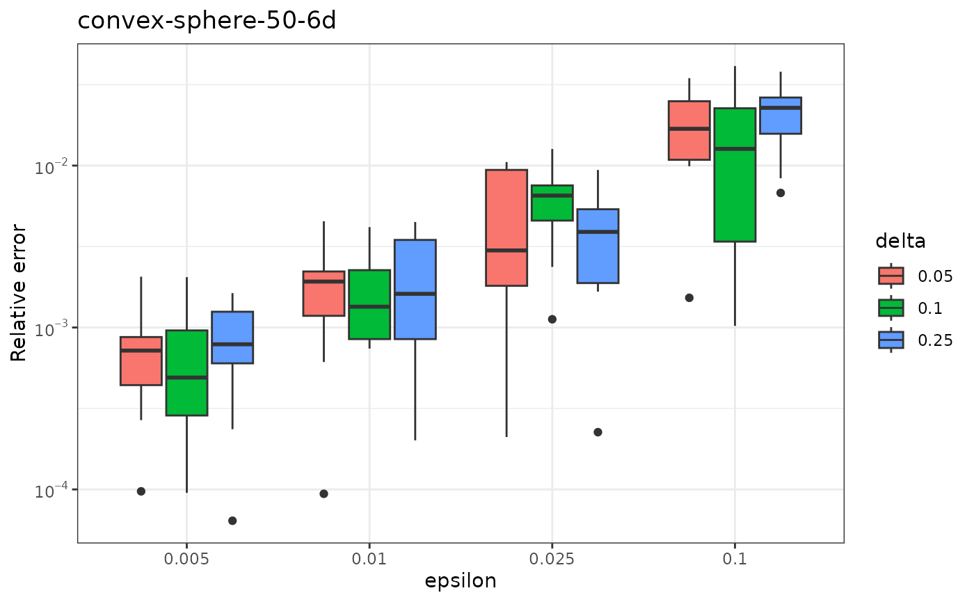

ggplot(res, aes(x = epsilon, y = time, color = delta, group = delta)) +
  stat_summary(fun = mean, geom = "line") +
  stat_summary(fun = mean, geom = "point") +
  scale_y_log10(labels = label_log()) +
  scale_x_discrete() +
  labs(y = "CPU time (s)") +
  ggtitle(paste0(shape, "-", npoints, "-", dim, "d")) +
  theme_bw()

References

Deng, Jingda, and Qingfu Zhang. 2019. “Approximating Hypervolume and Hypervolume Contributions Using Polar Coordinate.” IEEE Transactions on Evolutionary Computation 23 (5): 913–18. https://doi.org/10.1109/tevc.2019.2895108.

López-Ibáñez, Manuel. 2026. “Approximating the Hypervolume Indicator Using Fast Low-Discrepancy Sequences.” In Proceedings of the Genetic and Evolutionary Computation Conference, GECCO 2026, edited by Ting Hu and Leonardo Trujillo. ACM Press. https://doi.org/10.1145/3795095.3805198.