Empirical Attainment Function (EAF)

library(moocore)

The AUC of the EAF and the AOC (Hypervolume)

The Area-Over-the-Curve (i.e., the hypervolume) of a set of nondominated sets is exactly the the Area-Under-the-Curve (AUC) of their corresponding EAF (López-Ibáñez et al. 2025), as this example shows.

library(tidyr)
library(ggplot2)

extdata_dir <- system.file(package="moocore", "extdata")
A <- read_datasets(file.path(extdata_dir, "ALG_1_dat.xz"))
A[,1:2] <- normalise(A[,1:2], to_range = c(0,1))

aoc <- mean(sapply(split.data.frame(A[,1:2], A[,3]), hypervolume, reference = 1))
eaf_a <- eaf(A[,1:2], A[,3])
eaf_a[,3] <- eaf_a[,3]/100
auc <- hypervolume(eaf_a, reference = c(1,1,0), maximise = c(FALSE,FALSE,TRUE))
nruns <- length(unique(A[,3]))
cat("Runs = ", nruns,
    "\nAUC of EAF = ", auc,
    "\nMean AOC = ", aoc, "\n")
#> Runs =  90 
#> AUC of EAF =  0.7452171 
#> Mean AOC =  0.7452171

runs <- 5:nruns
aocs <- c()
aucs <- c()
for (r in runs) {
  a <- A[A[,3] <= r, ]
  aoc <- mean(sapply(split.data.frame(a[,1:2], a[,3]), hypervolume, reference = 1))
  eaf_a <- eaf(a[,1:2], a[,3])
  eaf_a[,3] <- eaf_a[,3]/100
  auc <- hypervolume(eaf_a, reference = c(1,1,0), maximise = c(FALSE,FALSE,TRUE))
  aocs <- c(aocs, aoc)
  aucs <- c(aucs, auc)
}

x <- tibble(r = runs, AOC = aocs, AUC=aucs) %>% pivot_longer(-r, names_to = "variable", values_to = "value")

ggplot(x, aes(r, value, color=variable, linetype=variable)) +
  geom_line(linewidth=1.5) +
  labs(x = "Number of sets", y = "Value", color = "", linetype="")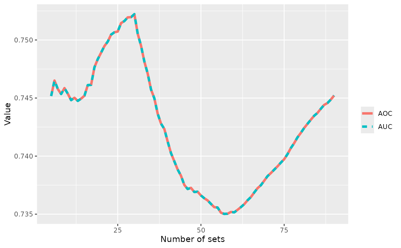

References

López-Ibáñez, Manuel, Diederick Vermetten, Johann Dreo, and Carola Doerr. 2025. “Using the Empirical Attainment Function for Analyzing Single-Objective Black-Box Optimization Algorithms.” IEEE Transactions on Evolutionary Computation. https://doi.org/10.1109/TEVC.2024.3462758.