This example illustrates how to sample random sets with mutually nondominated points.
Random nondominated sets in 2D
n <- 100
methods <- c("simplex", "concave-sphere", "convex-sphere", "convex-simplex",
"inverted-simplex", "concave-simplex")
colors <- c("red", "blue", "green", "purple", "orange", "yellow")
shapes <- c(16, 15, 17, 18, 16, 15) # ggplot2 shape codes
df_all <- do.call(rbind.data.frame, lapply(methods, function(method) {
points <- moocore::generate_ndset(n, 2, method = method, seed = 42)
data.frame(x = points[,1L], y = points[,2L], method = method)
}))
ggplot(df_all, aes(x = x, y = y, color = method, shape = method)) +
geom_point(size = 2) +
scale_color_manual(values = colors) +
scale_shape_manual(values = shapes) +
theme_minimal() +
labs(x = expression(z[1]), y = expression(z[2]),
title = "Random Nondominated Sets (2D)")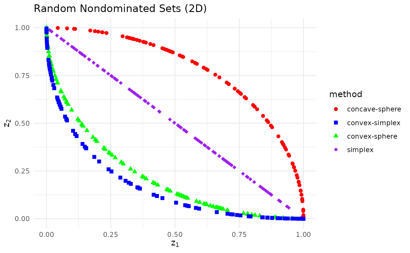
Random nondominated sets in integer space
We can also generate points in integer space.
points_list <- lapply(methods, function(method) {
moocore::generate_ndset(n, 2, method = method, seed = 42, integer = TRUE)
})
max_list <- sapply(points_list, max)
maximum <- max(max_list)
df_int <- do.call(rbind, lapply(seq_along(points_list), function(i) {
x <- points_list[[i]]
if (max_list[i] < maximum)
x <- moocore::normalise(x, lower = 0, upper = max_list[i], to_range = c(0, maximum))
data.frame(x = x[,1], y = x[,2], method = methods[i])
}))
ggplot(df_int, aes(x = x, y = y, color = method, shape = method)) +
geom_point(size = 2) +
scale_color_manual(values = colors) +
scale_shape_manual(values = shapes) +
theme_minimal() +
labs(x = expression(z[1]), y = expression(z[2]),
title = "Random Nondominated Sets in Integer Space (2D)")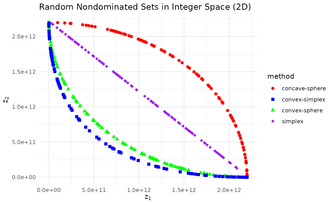
Variants of convex nondominated sets
A popular way to generate a convex nondominated set is to translate
the negative orthant of the hyper-sphere to the unit hyper-cube
(convex-sphere). However, there are other possible convex
sets with different properties. For example the method
convex-simplex squares the points generated by method
simplex, resulting in a convex transformation of the
standard simplex.
(show plotting code)
library(moocore)
library(htmltools)
library(plotly, warn.conflicts = FALSE)
plot_3d <- function(what, x, title) {
p <- plot_ly()
if (what == "simplex") {
# 2-simplex mesh
x_s <- diag(3)
p <- p %>% add_trace(
type = "mesh3d",
x = x_s[, 1L],
y = x_s[, 2L],
z = x_s[, 3L],
i = 0, j = 1, k = 2,
color = "cyan",
opacity = 0.2,
flatshading = TRUE,
name = "Simplex"
)
} else if (what %in% c("concave", "convex")) {
n_grid <- 50
phi <- seq(0, pi/2, length.out = n_grid)
theta <- seq(0, pi/2, length.out = n_grid)
grid <- expand.grid(phi = phi, theta = theta)
x_s <- matrix(sin(grid$phi) * cos(grid$theta), nrow = n_grid)
y_s <- matrix(sin(grid$phi) * sin(grid$theta), nrow = n_grid)
z_s <- matrix(cos(grid$phi), nrow = n_grid)
if (what == "convex") {
x_s <- 1 - x_s
y_s <- 1 - y_s
z_s <- 1 - z_s
}
p <- p %>% add_surface(
x = x_s,
y = y_s,
z = z_s,
colorscale = list(c(0, "cyan"), c(1, "cyan")),
opacity = 0.2,
showscale = FALSE
)
}
# Add scatter points
p <- p %>% add_trace(
type = "scatter3d",
mode = "markers",
x = x[, 1L],
y = x[, 2L],
z = x[, 3L],
marker = list(size = 2, color = "blue")
)
# Layout
p %>% layout(
title = title,
scene = list(
xaxis = list(title = "Z1", range = c(0,1)),
yaxis = list(title = "Z2", range = c(0,1)),
zaxis = list(title = "Z3", range = c(0,1)),
camera = list(eye = list(x = 1.2, y = 1.2, z = 0.8))
),
margin = list(l = 0, r = 0, b = 0, t = 40),
showlegend = FALSE
)
}
plotly_side_by_side <- function(fig1, fig2, height="500px") {
browsable(
tags$div(style="display:flex; justify-content: space-between;",
tags$div(style=sprintf("width:49%%; height:%s;", height),
plotly::as_widget(fig1)),
tags$div(style=sprintf("width:49%%; height:%s;", height),
plotly::as_widget(fig2))))
}
n <- 2000
fig1 <- plot_3d("simplex", moocore::generate_ndset(n, 3, "convex-sphere", seed = 42), title = 'method="convex-sphere"')
fig2 <- plot_3d("simplex", moocore::generate_ndset(n, 3, "convex-simplex", seed = 42), title = 'method="convex-simplex"')
plotly_side_by_side(fig1, fig2)The method convex-simplex implemented in
moocore::generate_ndset() is different from the
concave method proposed by Bringmann and
Friedrich (2012).
n <- 2000
points <- matrix(abs(rnorm(n * 3)), n, 3)
points <- points / (rowSums(sqrt(points)))^2
fig1 <- plot_3d("simplex", points, title = 'concave (Bringmann & Friedrich, 2012)')
plotly_side_by_side(fig1, fig2)Inverted shapes
Ishibuchi et al. (2019) analyze the differences
between regular and inverted shapes, shown below on
the left and right figures, respectively. The differences between
simplex and inverted-simplex are not
noticeable in 2D, but are significant in higher dimensions.
n <- 2000
fig1 <- plot_3d("simplex", moocore::generate_ndset(n, 3, "simplex", seed = 42), title = 'method="simplex"')
fig2 <- plot_3d("simplex", moocore::generate_ndset(n, 3, "inverted-simplex", seed = 42), title = 'method="inverted-simplex"')
plotly_side_by_side(fig1, fig2)
fig1 <- plot_3d("simplex", moocore::generate_ndset(n, 3, "concave-sphere", seed = 42), title = 'method="concave-sphere"')
fig2 <- plot_3d("simplex", moocore::generate_ndset(n, 3, "convex-sphere", seed = 42), title = 'method="convex-sphere"')
plotly_side_by_side(fig1, fig2)
fig1 <- plot_3d("simplex", moocore::generate_ndset(n, 3, "convex-simplex", seed = 42), title = 'method="convex-simplex"')
fig2 <- plot_3d("simplex", moocore::generate_ndset(n, 3, "concave-simplex", seed = 42), title = 'method="concave-simplex"')
plotly_side_by_side(fig1, fig2)Uniform sampling (moocore) vs projections of uniform samples (naive)
Naive methods for sampling such sets usually sample points uniformly in the hypercube and project them into a lower dimensional manifold (Lacour et al. 2017), e.g., the standard simplex or the positive orthant of the hypersphere. However, such projections do not preserve the uniformity of the sampling, that is, not all points in the manifold have the same probability of being sampled.
The function moocore::generate_ndset() produces a
uniform sampling on the manifold, as shown in the following
examples:
n <- 2000
# Simplex
points_moocore <- moocore::generate_ndset(n, 3, "simplex", seed = 42)
points_naive <- matrix(runif(n * 3), n, 3)
points_naive <- points_naive / rowSums(points_naive)
fig1 <- plot_3d("simplex", points_moocore, title = "Simplex (moocore)")
fig2 <- plot_3d("simplex", points_naive, title = "Simplex (naive)")
plotly_side_by_side(fig1, fig2)
# Concave-sphere
points_moocore <- moocore::generate_ndset(n, 3, "concave-sphere", seed = 42)
points_naive <- matrix(runif(n * 3), n, 3)
points_naive <- points_naive / sqrt(rowSums(points_naive^2))
fig1 <- plot_3d("concave", points_moocore, title = "Concave-sphere (moocore)")
fig2 <- plot_3d("concave", points_naive, title = "Concave-sphere (naive)")
plotly_side_by_side(fig1, fig2)
# Convex-sphere
points_moocore <- moocore::generate_ndset(n, 3, "convex-sphere", seed = 42)
points_naive <- 1 - points_naive
fig1 <- plot_3d("convex", points_moocore, title = "Convex-sphere (moocore)")
fig2 <- plot_3d("convex", points_naive, title = "Convex-sphere (naive)")
plotly_side_by_side(fig1, fig2)