Computing Multi-Objective Quality Metrics • moocore

Several examples of computing multi-objective unary quality metrics.

library(moocore)
library(dplyr, warn.conflicts=FALSE)
get_dataset <- function(filename)
  read_datasets(system.file(file.path("extdata", filename),
    package = "moocore", mustWork = TRUE))
apply_within_sets <- function(x, sets, FUN, ...) {
  FUN <- match.fun(FUN)
  sapply(X = split.data.frame(x, sets), FUN = FUN, ...)
}

Comparing two multi-objective datasets using unary quality metrics

First, read the datasets:

spherical <- get_dataset("spherical-250-10-3d.txt")
uniform <- get_dataset("uniform-250-10-3d.txt")

spherical_objs <- spherical[, -ncol(spherical)]
spherical_sets <- spherical[, ncol(spherical)]
uniform_objs <- uniform[, -ncol(uniform)] / 10
uniform_sets <- uniform[, ncol(uniform)]

Create reference set and reference point:

ref_set <- filter_dominated(rbind(spherical_objs, uniform_objs))
ref_point <- 1.1

Calculate metrics:

uniform_igd_plus <- apply_within_sets(uniform_objs, uniform_sets,
  igd_plus, ref = ref_set)
spherical_igd_plus <- apply_within_sets(spherical_objs, spherical_sets,
  igd_plus, ref = ref_set)

uniform_epsilon <- apply_within_sets(uniform_objs, uniform_sets,
  epsilon_mult, ref = ref_set)
spherical_epsilon <- apply_within_sets(spherical_objs, spherical_sets,
  epsilon_mult, ref = ref_set)

uniform_hypervolume <- apply_within_sets(uniform_objs, uniform_sets,
  hypervolume, ref = ref_point)
spherical_hypervolume <- apply_within_sets(spherical_objs, spherical_sets,
  hypervolume, ref = ref_point)

knitr::kable(data.frame(
  Uniform = c(mean(uniform_hypervolume), mean(uniform_igd_plus),
    mean(uniform_epsilon)),
  Spherical = c(mean(spherical_hypervolume), mean(spherical_igd_plus),
    mean(spherical_epsilon)),
  row.names = c("Mean HV","Mean IGD+","Mean eps*")), format = "html") %>%
  kableExtra::kable_styling(position = "center",
    bootstrap_options = c("striped", "condensed", "responsive"))

	Uniform	Spherical
Mean HV	0.7868862	0.7328974
Mean IGD+	0.1238303	0.1574521
Mean eps*	623.2775539	225.9158914

IGD and Average Hausdorff are not Pareto-compliant

Example 4 by Ishibuchi et al. (2015) shows a case where IGD gives the wrong answer:

ref <- matrix(c(10, 0, 6, 1, 2, 2, 1, 6, 0, 10), ncol = 2, byrow=TRUE)
A <- matrix(c(4, 2, 3, 3, 2, 4), ncol = 2, byrow=TRUE)
B <- matrix(c(8, 2, 4, 4, 2, 8), ncol = 2, byrow=TRUE)

par(mar = c(4, 4, 1, 1)) # Reduce empty margins
plot(ref, xlab=expression(f[1]), ylab=expression(f[2]),
  panel.first=grid(nx=NULL), pch=23, bg="gray", cex=1.5)
points(A, pch=1, cex=1.5)
points(B, pch=19, cex=1.5)
legend("topright", legend=c("Reference", "A", "B"), pch=c(23,1,19),
  pt.bg="gray", bg="white", bty = "n", pt.cex=1.5, cex=1.2)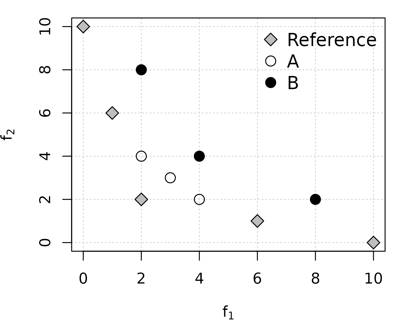

Assuming minimization of both objectives, $A$ is better than $B$ in terms of Pareto optimality. However, both igd() and avg_hausdorff_dist() incorrectly measure $B$ as better than $A$ , whereas igd_plus() and hypervolume() correctly measure $A$ as better than $B$ (remember that hypervolume must be maximized) and epsilon_additive() measures both as equally good (epsilon is weakly Pareto compliant).

knitr::kable(
  data.frame(
    A = c(
        igd(A, ref),
        avg_hausdorff_dist(A, ref),
        igd_plus(A, ref),
        epsilon_additive(A, ref),
        hypervolume(A, ref=10)),
    B = c(
        igd(B, ref),
        avg_hausdorff_dist(B, ref),
        igd_plus(B, ref),
        epsilon_additive(B, ref),
        hypervolume(B, ref=10)),
    row.names=c("IGD", "Hausdorff", "IGD+", "eps+", "HV")), format = "html") %>%
  kableExtra::kable_styling(position = "center",
    bootstrap_options = c("striped", "condensed", "responsive"))

	A	B
IGD	3.707092	2.591483
Hausdorff	3.707092	2.591483
IGD+	1.482843	2.260113
eps+	2.000000	2.000000
HV	61.000000	44.000000

References

Ishibuchi, Hisao, Hiroyuki Masuda, Yuki Tanigaki, and Yusuke Nojima. 2015. “Modified Distance Calculation in Generational Distance and Inverted Generational Distance.” In Evolutionary Multi-Criterion Optimization, EMO 2015 Part I, edited by António Gaspar-Cunha, Carlos Henggeler Antunes, and Carlos A. Coello Coello, 9018:110–25. Lecture Notes in Computer Science. Heidelberg, Germany: Springer.