hv_approx#
- moocore.hv_approx(points, /, ref, *, maximise=False, nsamples=262144, seed=None, method='Rphi-FWE+')[source]#
Approximate the hypervolume indicator.
Approximate the value of the hypervolume metric with respect to a given reference point assuming minimization of all objectives. Methods
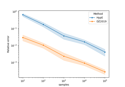
"Rphi-FWE+"and"DZ2019-HW"are deterministic and ignore the parameterseed, whilemethod="DZ2019-MC"relies on Monte-Carlo sampling [1]. All methods tend to get more accurate with higher values ofnsamples, but the increase in accuracy is not monotonic as shown in the example Comparing methods for approximating the hypervolume.See also
For details of the calculation, see the Notes section below.
- Parameters:
points (
ArrayLike) – Array of numerical values, where each row gives the coordinates of a point in objective space. If the array is created by theread_datasets()function, remove the last column.ref (
ArrayLike) – Reference point as a 1D vector. Must be either a single value, which will be used for all coordinates, or the same length as a single point inpoints.maximise (
bool|Sequence[bool], default:False) – Whether the objectives must be maximised instead of minimised. Either a single boolean value that applies to all objectives or a list of boolean values, with one value per objective. Also accepts a 1D numpy array with value 0/1 for each objective.nsamples (
int, default:262144) – Number of samples for Monte-Carlo sampling. Higher values typically produce more accurate approximations of the true hypervolume, but require more time.seed (
int|Generator|None, default:None) – Either an integer to seednumpy.random.default_rng(), Numpy default random number generator (RNG) or an instance of a Numpy-compatible RNG.Noneuses the equivalent of a random seed, as innumpy.random.default_rng().method (
Literal['DZ2019-HW','DZ2019-MC','Rphi-FWE+'], default:'Rphi-FWE+') – Method to approximate the hypervolume.
- Returns:
float– A single numerical value, the approximate hypervolume indicator.
See also
Notes
All available methods approximate the hypervolume as a \((m-1)\)-dimensional integral over the surface of hypersphere [1]:
\[\widehat{HV}_r(A) = \frac{2\pi^\frac{m}{2}}{\Gamma(\frac{m}{2})}\frac{1}{m 2^m}\frac{1}{n}\sum_{i=1}^n \max_{y \in A} s(w^{(i)}, y)^m\]where \(m\) is the number of objectives, \(w^{(i)}\) are weights uniformly distributed on \(S_{+}\), i.e., the positive orthant of the \((m-1)\)-D unit hypersphere, \(n\) is the number of weights sampled, \(\Gamma()\) is the gamma function
math.gamma(), i.e., the analytical continuation of the factorial function, and \(s(w, y) = \min_{k=1}^m (r_k - y_k)/w_k\).In the default
method="Rphi-FWE+"[2], the weights \(w^{(i)}, i=1\ldots n\) are defined using the deterministic low-discrepancy sequence \(R_\phi\) [3] mapped to the positive orthant of the hypersphere using a modified version of Fang and Wang efficient mapping [4].In
method="DZ2019-HW"[1], the weights \(w^{(i)}, i=1\ldots n\) are defined using a deterministic low-discrepancy sequence. The weight values depend on their number (nsamples), thus increasing the number of weights may not necessarily increase accuracy because the set of weights would be different.In
method="DZ2019-MC"[1], the weights \(w^{(i)}, i=1\ldots n\) are sampled from the unit normal vector such that each weight \(w = \frac{|x|}{\|x\|_2}\) where each component of \(x\) is independently sampled from the standard normal distribution [5].The original source code in C++/MATLAB for both
"DZ2019-HW"and"DZ2019-MC"methods can be found here.López-Ibáñez[2] empirically shows that
"Rphi-FWE+"typically produces an approximation error as low as the other methods, with a computational cost similar to"DZ2019-MC"and significantly faster than"DZ2019-HW".References
Examples
>>> x = np.array([[5, 5], [4, 6], [2, 7], [7, 4]])
>>> moocore.hypervolume(x, ref=[10, 10])
38.0
>>> moocore.hv_approx(x, ref=[10, 10], method="Rphi-FWE+")
37.99998
>>> moocore.hv_approx(x, ref=[10, 10], method="DZ2019-HW")
37.99996
>>> moocore.hv_approx(x, ref=[10, 10], seed=42, method="DZ2019-MC")
38.00081
Merge all the sets of a dataset by removing the set number column:
>>> x = moocore.get_dataset("input1.dat")[:, :-1]
Dominated points are ignored, so this:
>>> moocore.hv_approx(x, ref=10)
93.5533
>>> moocore.hv_approx(x, ref=10, method="DZ2019-HW")
93.5533
gives the same hypervolume approximation as this:
>>> x = moocore.filter_dominated(x)
>>> moocore.hv_approx(x, ref=10)
93.5533
>>> moocore.hv_approx(x, ref=10, method="DZ2019-HW")
93.5533
The approximation is far from perfect for large number of dimensions:
>>> x = moocore.get_dataset("ran.10pts.9d.10")[:, :-1]
>>> x = moocore.filter_dominated(-x, maximise=True)
>>> x = moocore.normalise(x, to_range=[1, 2])
>>> reference = 0.9
>>> moocore.hypervolume(x, ref=reference, maximise=True)
0.483633123747
>>> moocore.hv_approx(x, ref=reference, maximise=True)
0.48397532301
>>> moocore.hv_approx(x, ref=reference, maximise=True, method="DZ2019-HW")
0.483083547763
Gallery examples#
Comparing methods for approximating the hypervolume