Comparing methods for approximating the hypervolume

The following examples compare various ways of approximating the hypervolume of a nondominated set.

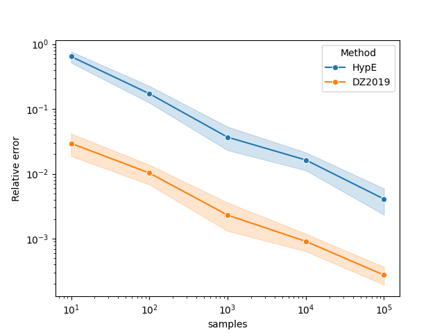
Comparing HypE and Rphi-FWE+

This example shows how to approximate the hypervolume metric of the CPFs.txt dataset using both moocore.whv_hype() (HypE), and moocore.hv_approx() for several values of the number of samples between \(10^1\) and \(10^5\). We repeat each calculation 5 times to account for stochasticity.

import numpy as np
import pandas as pd
import matplotlib.pyplot as plt
import seaborn as sns
import moocore

First calculate the exact hypervolume.

ref = 2.1
x = moocore.get_dataset("CPFs.txt.xz")[:, :-1]
x = moocore.filter_dominated(x)
x = moocore.normalise(x, to_range=[1, 2])
true_hv = moocore.hypervolume(x, ref=ref)

Next, we approximate the hypervolume using \(\{10^1, 10^2, \ldots, 10^5\}\) random samples to show the higher samples reduce the approximation error. Since the approximation is stochastic, we perform 5 repetitions of each computation.

nreps = 5
nsamples_exp = 5
rng1 = np.random.default_rng(42)
rng2 = np.random.default_rng(42)
results = []
for i in range(1, nsamples_exp + 1):
    for r in range(nreps):
        res = moocore.whv_hype(x, ref=ref, ideal=0, nsamples=10**i, seed=rng1)
        results.append(dict(Method="HypE", rep=r, samples=i, value=res))
        res = moocore.hv_approx(
            x, ref=ref, nsamples=10**i, seed=rng2, method="DZ2019-MC"
        )
        results.append(dict(Method="DZ2019-MC", rep=r, samples=i, value=res))

    res = moocore.hv_approx(x, ref=ref, nsamples=10**i, method="DZ2019-HW")
    results.append(dict(Method="DZ2019-HW", rep=0, samples=i, value=res))
    res = moocore.hv_approx(x, ref=ref, nsamples=10**i, method="Rphi-FWE+")
    results.append(dict(Method="Rphi-FWE+", rep=0, samples=i, value=res))


width = len("Mean DZ2019-MC")
text = "True HV"
print(f"{text:>{width}} : {true_hv:.5f}")
df = pd.DataFrame(results)
df["Method"] = (
    df["Method"]
    .astype("category")
    .cat.reorder_categories(["DZ2019-MC", "DZ2019-HW", "Rphi-FWE+", "HypE"])
)
subdf = (
    df[df["samples"] == 4]
    .groupby("Method", observed=True)["value"]
    .agg(["mean", "min", "max"])
)
for what, mean, min, max in subdf.itertuples():
    text = "Mean " + what
    print(f"{text:>{width}} : {mean:.5f} [{min:.5f}, {max:.5f}]")

       True HV : 1.05704
Mean DZ2019-MC : 1.05766 [1.05579, 1.06019]
Mean DZ2019-HW : 1.05704 [1.05704, 1.05704]
Mean Rphi-FWE+ : 1.05703 [1.05703, 1.05703]
     Mean HypE : 1.07701 [1.04252, 1.11705]

Next, we plot the results.

df["samples"] = 10 ** df["samples"]
df["value"] = np.abs(df["value"] - true_hv) / true_hv

ax = sns.lineplot(x="samples", y="value", hue="Method", data=df, marker="o")
ax.set(xscale="log", yscale="log", ylabel="Relative error")
plt.show()

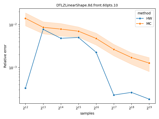
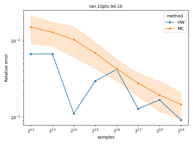
Comparing Monte-Carlo and quasi-Monte-Carlo approximations

The quasi-Monte-Carlo approximations with method="Rphi-FWE+" ^[13] and method="DZ2019-HW" ^[12] is deterministic, but not monotonic on the number of samples. Nevertheless, they are often better than the Monte-Carlo approximation produced by method="DZ2019-MC" ^[12], specially with large number of objectives. A more detailed comparison is provided by López-Ibáñez^[13].

datasets = ["DTLZLinearShape.8d.front.60pts.10", "ran.10pts.9d.10"]
ref = 10
samples = 2 ** np.arange(12, 19)
maxiter = samples.max()

for dataset in datasets:
    x = moocore.get_dataset(dataset)[:, :-1]
    x = moocore.filter_dominated(x)
    exact = moocore.hypervolume(x, ref=ref)

    res = []
    for i in samples:
        hv = moocore.hv_approx(x, ref=ref, nsamples=i, method="DZ2019-HW")
        res.append(dict(samples=i, method="DZ2019-HW", hv=hv))
        hv = moocore.hv_approx(x, ref=ref, nsamples=i, method="Rphi-FWE+")
        res.append(dict(samples=i, method="Rphi-FWE+", hv=hv))
        for k in range(5):
            hv = moocore.hv_approx(
                x, ref=ref, nsamples=i, method="DZ2019-MC", seed=k
            )
            res.append(dict(samples=i, method="DZ2019-MC", hv=hv))

    df = pd.DataFrame(res)
    df["hverror"] = np.abs(1.0 - (df.hv / exact))
    df["method"] = (
        df["method"]
        .astype("category")
        .cat.reorder_categories(["DZ2019-MC", "DZ2019-HW", "Rphi-FWE+"])
    )

    plt.figure()
    ax = sns.lineplot(
        data=df, x="samples", y="hverror", hue="method", marker="o"
    )
    ax.set_title(f"{dataset}", fontsize=10)
    ax.set(yscale="log", ylabel="Relative error")
    ax.set_xscale("log", base=2)
    plt.tight_layout()

plt.show()

• 
•