Rank points according to Pareto-optimality (nondominated sorting).

pareto_rank() is meant to be used like rank(), but it assigns ranks according to Pareto dominance, where rank 1 indicates those solutions not dominated by any other solution in the input set. Duplicated points are assigned the same rank. The resulting ranking can be used to partition points into a list of matrices, each matrix representing a nondominated front (Deb et al. 2002) (see examples below).

Usage

pareto_rank(x, maximise = FALSE)

Arguments

x: matrix()|data.frame()
Matrix or data frame of numerical values, where each row gives the coordinates of a point.
maximise: logical()
Whether the objectives must be maximised instead of minimised. Either a single logical value that applies to all objectives or a vector of logical values, with one value per objective.

Value

An integer vector of the same length as the number of rows of the input x, where each value gives the rank of each point (lower is better).

Details

Given a finite set of points $X \subset \mathbb{R}^m$, the rank of a point $x \in X$ is defined as:

$$\operatorname{rank}(x) = r \iff x \in F^c_{r} \land \nexists y \in F^c_{r}, y \prec x$$

where $y \prec x$ means that $y$ dominates $x$ according to Pareto optimality, $F^c_r = X \setminus \bigcup_{i=1}^{r-1} F_i$ and $F_r = \{x \in X \land \operatorname{rank}(x) = r\}$. The sets $F_c$, with $c=1,\dots,k$, partition $X$ into $k$ fronts, that is, mutually nondominated subsets of $X$.

With $m=2$, i.e., ncol(data)=2, the code uses the best-known $O(n \log n)$ algorithm by Jensen (2003) . When $m \geq 3$, it uses the naive algorithm that identifies one front at a time, which requires $O(n^2\log n)$ for $m=3$, and $O(n^2 \log^{m-2} n)$ for $m \geq 4$.

References

Kalyanmoy Deb, A Pratap, S Agarwal, T Meyarivan (2002). “A fast and elitist multi-objective genetic algorithm: NSGA-II.” IEEE Transactions on Evolutionary Computation, 6(2), 182–197. doi:10.1109/4235.996017 .

M T Jensen (2003). “Reducing the run-time complexity of multiobjective EAs: The NSGA-II and other algorithms.” IEEE Transactions on Evolutionary Computation, 7(5), 503–515.

Examples

three_fronts = matrix(c(1, 2, 3,
                        3, 1, 2,
                        2, 3, 1,
                        10, 20, 30,
                        30, 10, 20,
                        20, 30, 10,
                        100, 200, 300,
                        300, 100, 200,
                        200, 300, 100), ncol=3, byrow=TRUE)
pareto_rank(three_fronts)
#> [1] 1 1 1 2 2 2 3 3 3

split.data.frame(three_fronts, pareto_rank(three_fronts))
#> $`1`
#>      [,1] [,2] [,3]
#> [1,]    1    2    3
#> [2,]    3    1    2
#> [3,]    2    3    1
#> 
#> $`2`
#>      [,1] [,2] [,3]
#> [1,]   10   20   30
#> [2,]   30   10   20
#> [3,]   20   30   10
#> 
#> $`3`
#>      [,1] [,2] [,3]
#> [1,]  100  200  300
#> [2,]  300  100  200
#> [3,]  200  300  100
#> 
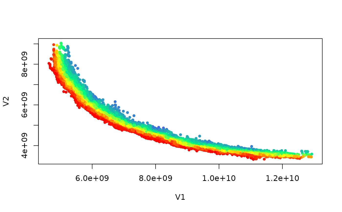
path_A1 <- file.path(system.file(package="moocore"),"extdata","ALG_1_dat.xz")
set <- read_datasets(path_A1)[,1:2]
ranks <- pareto_rank(set)
str(ranks)
#>  int [1:23260] 13 24 20 22 22 5 23 5 16 20 ...
if (requireNamespace("graphics", quietly = TRUE)) {
   colors <- colorRampPalette(c("red","yellow","springgreen","royalblue"))(max(ranks))
   plot(set, col = colors[ranks], type = "p", pch = 20)
}